In previous posts (Part 1 , Part 2) we talked about how to solve satellite imagery problems with NAS, and more specifically how we can do that with AutoKeras [1]. AutoKeras is a convenient, off-the-shelf NAS library with built-in functionality for deep learning tasks like classification and regression. However, we can use NAS for many other tasks, including low-level image tasks like super-resolution. In this post, we will show you how to do that, following the example from our recent paper [2].
Super-resolution
We need high-resolution imagery for many tasks, such as crop monitoring or building detection, but higher spatial resolution imagery might not be available or very expensive to obtain. Fortunately, we can increase the resolution of images using super-resolution (SR) techniques. The current state-of-the-art in super-resolution is deep learning. The design of super-resolution networks offers many challenges because the task determines what type of network you need. For example, maintaining sharp edges is imperative when your end goal is building detection. However, when your goal is crop monitoring, the spectral signatures are much more important. The manual design of the networks ensures that you can select the ideal network properties for your task. However, the problem is that SR is just one step in the pipeline: you still need to make many other choices, such as which model to use for the downstream task. This process of carefully selecting and crafting every step in the pipeline quickly becomes very time-consuming.
AutoSR4EO
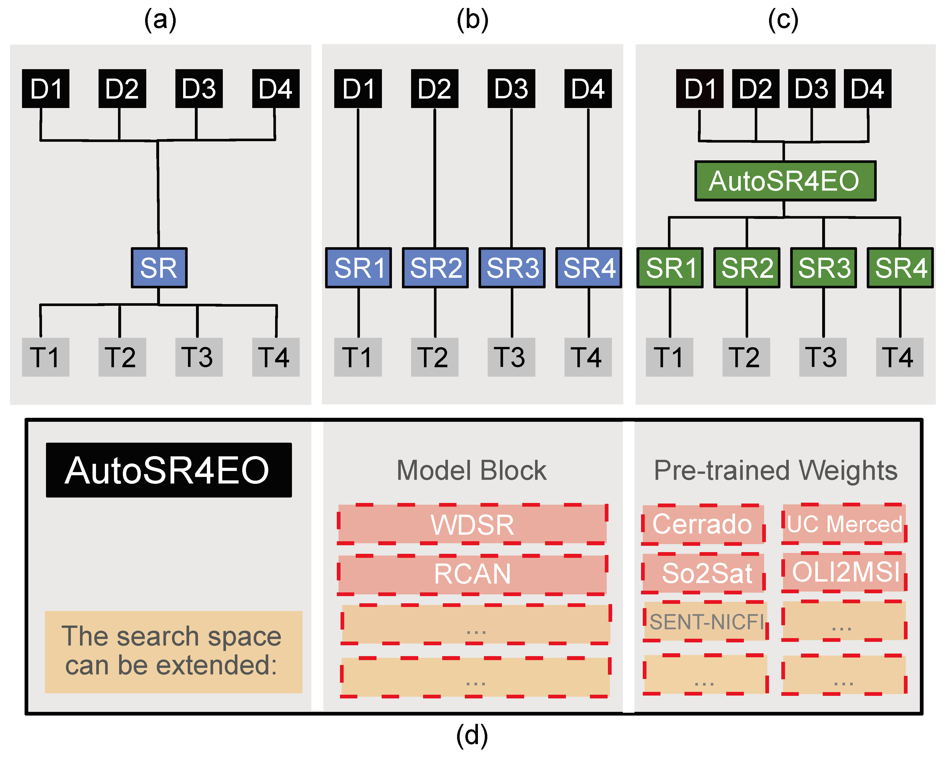
A promising solution to the problem of EO pipeline design is to automatically design SR neural networks using NAS (see previous posts for more details). NAS has multiple advantages. First of all, while performing a NAS search takes longer than training a single model, it can be much faster than designing models through trial and error. Second, automatic design is really convenient if you want to create a customised neural network architecture, but you might not yet have experience configuring neural networks. Finally, the intelligent search algorithms used in NAS systems find better results than humans could. For these reasons, we proposed an architecture-level NAS based on state-of-the-art neural networks, which extends AutoKeras with the task of SR, called AutoSR4EO [2]. Our methods exploit the modular architecture of modern neural networks. While many NAS approaches focus on designing these repeated modules, we use modules from expert-designed networks and use NAS to determine which type of module to stack, how many to stack, and which pre-trained weights to load. Our methods achieve the highest rank compared to state-of-the-art neural networks. Our framework can be easily extended with newer architectures by adding model blocks to the search space.
Figure 1. Top: Three options for designing SR networks: (a) we use a single, well-performing model for all cases, ignoring the requirements of specific tasks; (b) we select or design a network for each task, which takes a lot of time; (c) we use a NAS system like AutoSR4EO to design the ideal network for any given SR task. Bottom: The search space of AutoSR4EO consists of state-of-the-art model blocks and sets of pre-trained weights obtained from different satellite image datasets (Wasala et al. 2024) [2]
Implementation
We needed to make three significant modifications to AutoKeras to make AutoSR4EO possible: – We adjusted the AutoKeras source code to add two SR metrics: PSNR and SSIM. – We implemented a new SR “task head”. AutoKeras has a few built-in task heads, the final layers of the network that reshape the network features into the correct output shape for the task. While AutoKeras has regression and classification heads, none actually return an image, which you need for dense image tasks like SR and segmentation. We implemented a new search space based on SR networks. AutoKeras offers a few built-in search spaces, like the image classification task, which has blocks of convolutional layers but also full nets like Resnet or Xception. However, just like you need different metrics for different tasks, SR nets need different architectures, so we implemented new blocks based on SOTA SR networks.
*A note on the implementation*. We don’t give more details on the implementation in this blog because we implemented these changes in an older version of AutoKeras, and we have not tested these changes with the newer versions. While AutoKeras is very convenient off-the-shelf if you want to do one of the natively supported tasks, it can be tricky to customise it. You can see the code and the forked version of AutoKeras here and here. You can contact me for more details (j.wasala<at>liacs.leidenuniv.nl).
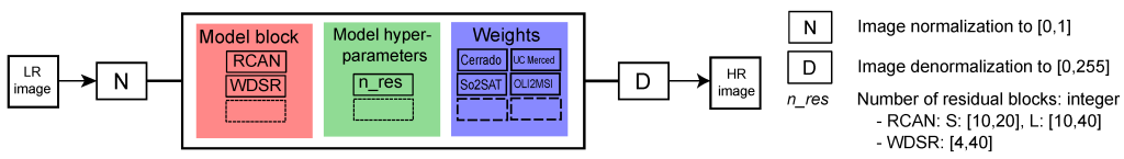
Caption:The search space of AutoSR4EO consists of (1) model blocks, (2) model depth and (3) choice of pre-trained weights. The implementation of the search space and network output and the addition of SR-specific metrics required significant modifications to the AutoKeras source code.
Towards a unified NAS for EO
AutoSR4EO shows that NAS can help us improve by automating network design for EO tasks. However, we have yet to have a single, unified NAS solution that would be able to solve many important EO tasks. Many existing NAS systems are designed for specific use cases (e.g., targeting a single problem or dataset), and convenient toolboxes like AutoKeras only cover a few deep learning tasks. These challenges limit the accessibility of NAS: either people cannot use it at all for their tasks, or they need to make significant modifications to their data, such as transforming it into a tabular format to use frameworks like AutoSklearn or AutoGluon. We need more research to develop NAS solutions for other tasks to make NAS, and by extension, deep learning, more accessible to researchers in high-impact fields like EO.
References
[1] Haifeng Jin, Qingquan Song, and Xia Hu. 2019. Auto-Keras: An Efficient Neural Architecture Search System. In Proceedings of the 25th ACM SIGKDD International Conference on Knowledge Discovery & Data Mining (KDD ’19). Association for Computing Machinery, New York, NY, USA, 1946–1956. https://doi.org/10.1145/3292500.3330648 
[2] Wąsala J, Marselis S, Arp L, Hoos H, Longépé N, Baratchi M. AutoSR4EO: An AutoML Approach to Super-Resolution for Earth Observation Images. Remote Sensing. 2024; 16(3):443. https://doi.org/10.3390/rs16030443
This year, we met again in person with the Optimisation and AutoML community at COSEAL in Paris at Sorbonne University. Our former group member, Koen van der Blom, co-hosted the event. We were very happy to see him again!
COSEAL was well-attended, with over 100 registered participants from the AutoML groups in Freiburg and Hannover, the organising LIP6, the Slovenian Jozef Stefan institute, and even from local companies like Huawei France, among others. In other words, Little Ada met a lot of new friends. Of course, ADA was well-represented as well: Holger, Mitra, Samira, Julia and Hadar were there. We were happy to find many of our friends and collaborators at COSEAL, including Frank Hutter, Marius Lindauer, Lars Kotthoff, Saso Dzeroski and former ADA member Jeroen.
COSEAL 2023 group picture. Can you spot the ADA members?
The first day, Julia gave her first academic talk on her work on AutoML for super-resolution, which she did for a master’s thesis. She also presented a poster on her current work on AutoML for methane plume detection (read more about it here). Hadar presented a poster on his master’s thesis work on Graph Neural Networks for SAT problems. The day ended on a (literal) high note, with a reception at the top of the tower of Sorbonne’s science faculty, with a beautiful view over Paris and, most notably, the Eifel tower.
The next day we had the opportunity to enjoy a long talk by Holger on the recent work on Neural Network Verification by Matthias and Annelot, which was rewarded with the best paper award at the AAAI Workshop on Safe AI. Samira presented yet another of our applications to AutoML to different fields by showcasing her work on AutoML for Radio Astronomy.
Finally, on Wednesday, Mitra gave a talk on AutoML for hybrid (physical) modelling in Earth Observation, a topic that Laurens and Nuno work on (Read more about Laurens’ work here, and Nuno’s work here [link upcoming]. Read the work by former master student Victor here).
After two and a half days of talks and presentations, it was time to say goodbye to COSEAL. Fortunately, some of us could stay to attend the AutoML workshop.
The AutoML workshop was a whole different event, focussed on discussions and exchanging ideas within the community. For two days, we had many fruitful discussions on topics including benchmarking, multi-objective optimisation, explainable and interactive AutoML, and ethics and fairness.
It was an exciting week, full of exchanges of research ideas and interesting discussions. A great success for ADA: we gave a peek into how varied our work in the field of AutoML is before returning to Leiden, a little tired but full of new ideas.
This is the second blog post in the series about our research on Neural Architecture Search (NAS) for Earth Observation (EO). In Part 1 we introduced NAS and how it can be applied to EO. We talked about a NAS framework: AutoKeras [1], and briefly discussed how it can be customized for EO tasks.
In this blog post, we talk about how AutoKeras can be used to create methods for EO imagery. More specifically, we are going to tackle the task of classification of EO imagery through the work “Automated Machine Learning for Satellite Data: Integrating Remote Sensing Pre-trained Models into AutoML Systems” by Nelly R. Palacios Salinas, Mitra Baratchi, Jan N. van Rijn and Andreas Vollrath [2]. It is the first work that focused on developing AutoML methods for EO.
Even though we will discuss how you could create methods like this yourself, Palacios et al. already present a framework for the classification of EO imagery that can be used with just a few lines of code and without requiring in-depth prior knowledge of AutoML or deep learning in general. The links to the code as well as the full Python notebook for this blog can be found at the end of the post.
Figure 1: Examples of images and labels in scene classification. Source: UC Merced [13]
Classification
Image classification is the task of assigning labels to an image. For instance, you’d like to know whether your image is showing a desert or a forest or some other type of land cover. Classification has, among others, applications in tasks like urban planning, hazard detection, and monitoring of the environment [3]. In EO the term “image classification” is sometimes used to refer to what is called segmentation in computer science. This is the task of assigning labels to individual pixels. For instance, this is the case when you classify pixels into the classes “building” or “not building” for building segmentation tasks. We, however, will only talk about classification in the traditional sense where you consider the complete image.
Figure 2: Example of segmentation or pixel classification: building footprint segmentation. The image on the left shows the input image, on the right you see the segmentation map where “building” pixels are white, and background pixels are black. Source
EO imagery
The task of classifying natural images is very different from the task of classifying EO images. In EO images, areas of interest can be very small on the image. For instance, if you want to differentiate between “savanna” and “bare ground”, individual plants could cover only a few pixels or less, depending on the resolution of the image. In some satellite images, like those obtained from Sentinel-2 with a resolution of 10 m per pixel, a plant could even be much smaller than a single pixel. Additionally, an EO image can cover a large area that includes multiple land cover types and can contain image features on different scales, from a tree covering a few pixels to larger patterns in the image like a lake. These properties need to be taken into account when designing NAS frameworks for the classification of EO imagery.
NAS for classification of EO imagery
Many NAS frameworks exist for the classification of natural images, including NASnet [4], AutoGAN [5], and ENAS [6]. Whereas these frameworks work exceptionally well for natural images, these have not been designed with the complexity of satellite imagery in mind, and therefore their performance and applications for EO data are limited. One of the main reasons for these limitations lay down in the use of datasets with simpler images like CIFAR-10 [6] for training and evaluation.
Currently, NAS methods are being developed specifically for classifying EO images. For instance, the work of our research group members Palacios Salinas et al. [2] shows that their classifier developed in AutoKeras is able to outperform 71% of the baseline methods created for natural images. These results were achieved by customizing AutoKeras’ ImageClassifier.
Classification in AutoKeras
AutoKeras has a ready-to-use NAS system for image classification, which is called the ImageClassifier. The search space of the ImageClassifier consists of various code modules that can be morphed, repeated, and combined to form a neural network. This type of AutoKeras block that can combine multiple types of blocks is called a hyperblock. The options include ResNet [7], Xception [8], and a convolutional block. It’s possible to use pre-trained weights from ImageNet [8], which is a natural image dataset. If you need a refresher on AutoKeras, read our previous blogpost on this topic.
Tutorial: Hyperblock
AutoKeras has documentation on how to implement your own blocks, but let’s take it a step further and take a look at how we can implement a hyperblock that will allow you to choose from different blocks. We’re going to implement a hyperblock that will let the NAS framework choose between ResNet and Xception.
import autokeras as ak
import tensorflow as tf

class HyperBlock(ak.Block):
    def build(self, hp, inputs):
        inputs = tf.nest.flatten(inputs)[0]

        if hp.Choice("model_type",["resnet", "xception"]) == "resnet":
            outputs = ak.ResNetBlock().build(hp,inputs)
        else:
            outputs=ak.XceptionBlock().build(hp,inputs)
        return outputs
Here we define a new class that builds either a ResNet or a DenseNet block. You can modify the HyperBlock to make it possible to choose which model you want beforehand:
from typing import Optional

class HyperBlock(ak.Block):
    def __init__(self, model_type: Optional[str] = None,**kwargs):
        super().__init__(**kwargs)

        if model_type is not None and model_type != "resnet" and model_type != "xception":
            raise Exception(f"invalid model_type {model_type}")

        self.model_type=model_type

    def get_config(self):
        config = super().get_config()
        config.update({"model_type": self.model_type})
        return config

    def _build_model(self,hp, output_node,model_type: str):
        if model_type=="resnet":
            return ak.ResNetBlock().build(hp,output_node)
        elif model_type=="xception":
            return ak.XceptionBlock().build(hp, output_node)

    def build(self, hp, inputs):
        inputs=tf.nest.flatten(inputs)[0]

        # Let AutoKeras choose a model
        if self.model_type is None:
            model_type= hp.Choice("model_type", ["resnet", "xception"])
            with hp.conditional_scope("model_type",[model_type]):
                outputs = self._build_model(hp,inputs,model_type)
        # Select model yourself
        else:
            outputs = self._build_model(hp,inputs,model_type)
As you can see, this becomes considerably more complicated. Let’s break down the changes:
We added an __init__ method so you can specify the model_type parameter
Error handling is important: check whether a valid model_type parameter has been passed
get_config: add the new block parameter to the config
build: because you now have 2 scenarios (let AutoKeras choose a model or select yourself), we now need a conditional scope. The value of model_type which is selected by AutoKeras, will now only be active within the scope.
_build_model: helper function to avoid code repetition. This becomes especially helpful if you have many options.
Here you go, your first hyperblock! You can also make your own block based on a specific neural network architecture and include it in your hyperblock. We will show you how to do this in Part 3 of this series.
Transfer learning
The ImageClassifier also gives you the option to use models that are pre-trained on ImageNet. However, as we discussed, this is not very useful for EO imagery (or even natural images, see: Rethinking Pre-training and Self-training [9]). Palacios Salinas et al. solved this by loading weights obtained from pre-training on some common EO datasets: RESISC45 [10], EUROSAT [11], So2SAT [12] and UC Merced [13].
Tutorial: loading weights
We’re going to look at how we can load these weights in our HyperBlock. Luckily for us, the weights can be downloaded from https://tfhub.dev.
Before we can use these weights in our HyperBlock, we need to make a ResNet block that can load the weights.
import tensorflow_hub as hub

class EOResNetBlock(ak.Block):
    #Remote sensing pretrained modules based on: https://github.com/palaciosnrps/automl-rs-project/blob/714bbe36c68fd0f2b989bfee89eac9497d7acf45/autokeras/blocks/basic.py"""
    def __init__(
         self,
         version: Optional[str] = None,
         **kwargs,
         ):
            super().__init__(**kwargs)

            if version is not None and version not in EO_VERSIONS.keys() and set(version) <= set(EO_VERSIONS.keys()):
                raise Exception(f"invalid version {version}")

            self.version=version

    def get_config(self):
        config = super().get_config()
        config.update({"version": self.version})
        return config

    def build(self, hp, inputs=None):
        input_node = tf.nest.flatten(inputs)[0]

        if self.version is None:
            version= hp.Choice("version", list(EO_VERSIONS.keys()))
        elif isinstance(self.version,list):
            version = self.version
        else:
            version = [self.version]

        module = hub.KerasLayer(EO_VERSIONS[version],tags='train',trainable=False)
        min_size = 224
        if input_node.shape[3] not in [1, 3]:
            if self.pretrained:
                raise ValueError(
                    "When pretrained is set to True, expect input to "
                    "have 1 or 3 channels, bug got "
                    "{channels}.".format(channels=input_node.shape[3])
                )

        if input_node.shape[1] < min_size or input_node.shape[2] < min_size:
            input_node = tf.keras.layers.experimental.preprocessing.Resizing(
                max(min_size, input_node.shape[1]),
                max(min_size, input_node.shape[2]),
            )(input_node)
        if input_node.shape[3] == 1:
            input_node = tf.keras.layers.Concatenate()([input_node] * 3)
        if input_node.shape[3] != 3:
            input_node = tf.keras.layers.Conv2D(filters=3, kernel_size=1, padding="same")(
                input_node
            )

        output_node = module(input_node)
        return output_node
In fact, this block is very similar to the HyperBlock, but instead of model_type it has a version parameter that specifies which weights to use. Once again, we check whether a correct version has been specified by the user. The build function is a bit different:
We do not need a conditional scope now, because we don’t build blocks in a conditional statement.
A module is created that serves as an interface to pre-trained tensorflow models.
The number of channels of the input data is checked to make sure it agrees with the pre-trained model.
Now we can add our pre-trained block to the HyperBlock:
class HyperBlock(ak.Block):
    def __init__(self, model_type: Optional[str] = None, version: Optional[str] = None,**kwargs):
        super().__init__(**kwargs)

        if model_type is not None and model_type != "resnet" and model_type != "xception" and model_type != "eo_resnet":
            raise Exception(f"invalid model_type {model_type}")

        self.model_type=model_type
        self.version = version

    def get_config(self):
        config = super().get_config()
        config.update({"model_type": self.model_type})
        return config

    def _build_model(self,hp, output_node,model_type: str):
        if model_type=="resnet":
            return ak.ResNetBlock().build(hp,output_node)
        elif model_type=="xception":
            return ak.XceptionBlock().build(hp, output_node)
        elif model_type=="eo_resnet":
            return EOResNetBlock(version=self.version).build(hp,output_node)

    def build(self, hp, inputs):
        inputs=tf.nest.flatten(inputs)[0]

        # Let AutoKeras choose a model
        if self.model_type is None:
            model_type= hp.Choice("model_type", ["resnet", "xception", "eo_resnet"])
            with hp.conditional_scope("model_type",[model_type]):
                outputs = self._build_model(hp,inputs,model_type)
        # Select model yourself
        else:
            outputs = self._build_model(hp,inputs,self.model_type)
        return outputs
We can use our block to create a custom NAS with the AutoModel class of AutoKeras and train it on the UC Merced dataset. The number of trials determines how many networks are sampled by AutoKeras. We now set it to 1, just to test whether it works.
import tensorflow_datasets as tfds
# load the dataset 317.MiB
train_set=tfds.as_numpy(tfds.load("uc_merced", download=True,as_supervised=False, batch_size=-1,split="train[:80%]"))
test_set=tfds.as_numpy(tfds.load("uc_merced", download=True,as_supervised=False, batch_size=-1,split="train[80%:]"))

weights_versions = {k: v for k,v in EO_VERSIONS.items() if k != "ucmerced"}

input_node = ak.ImageInput()
output_node = HyperBlock(model_type="eo_resnet")(input_node)
output_node = ak.ClassificationHead()(output_node)
eo_nas_model = ak.AutoModel(input_node, output_node, max_trials=1,overwrite=True)

eo_nas_model.fit(x=train_set["image"], y=train_set["label"], epochs=10)
When you run this, you’ll find that the model compiles and the neural architecture search starts. Success!
Conclusion
In this blog post, we discussed NAS for the classification of EO images. Using the work by Palacios Salinas et al. as an example, you have learned how to customize the AutoKeras search space by creating a hyperblock and how to apply transfer learning by including pre-trained weights obtained from training on EO datasets.
In the next post, we will go even further into the customization of AutoKeras with another example of our research: NAS for super-resolution. We’re going to cover how to add our own custom metrics, add new model architectures to the search space, and extend AutoKeras to other tasks. Stay tuned for more advanced tutorials on AutoKeras for EO!
References
[1] Jin, H., Song, Q. and Hu, X., 2019, July. Auto-keras: An efficient neural architecture search system. In Proceedings of the 25th ACM SIGKDD international conference on knowledge discovery & data mining (pp. 1946-1956).
[2] Palacios Salinas, N.R., Baratchi, M., Rijn, J.N.V. and Vollrath, A., 2021, September. Automated machine learning for satellite data: integrating remote sensing pre-trained models into AutoML systems. In Joint European Conference on Machine Learning and Knowledge Discovery in Databases (pp. 447-462). Springer, Cham.
[3] Cheng, G., et al.: Remote sensing image scene classification meets deep learning: Challenges, methods, benchmarks, and opportunities. In: IEEE Journal of Selected Topics in Applied Earth Observations and Remote Sensing 13, 3735–3756 (2020)
[4] Zoph, B., Vasudevan, V., Shlens, J. and Le, Q.V., 2018. Learning transferable architectures for scalable image recognition. In Proceedings of the IEEE conference on computer vision and pattern recognition (pp. 8697-8710).
[5] Gong, X., Chang, S., Jiang, Y. and Wang, Z., 2019. Autogan: Neural architecture search for generative adversarial networks. In Proceedings of the IEEE/CVF International Conference on Computer Vision (pp. 3224-3234).
[6] Pham, H., Guan, M., Zoph, B., Le, Q. and Dean, J., 2018, July. Efficient neural architecture search via parameters sharing. In International conference on machine learning (pp. 4095-4104). PMLR.
[7] He, K., Zhang, X., Ren, S. and Sun, J., 2016. Deep residual learning for image recognition. In Proceedings of the IEEE conference on computer vision and pattern recognition (pp. 770-778).
[8] Chollet, F., 2017. Xception: Deep learning with depthwise separable convolutions. In Proceedings of the IEEE conference on computer vision and pattern recognition (pp. 1251-1258).
[9] Zoph, B., Ghiasi, G., Lin, T.Y., Cui, Y., Liu, H., Cubuk, E.D. and Le, Q., 2020. Rethinking pre-training and self-training. Advances in neural information processing systems, 33, pp.3833-3845.
[10] Cheng, G., Han, J. and Lu, X., 2017. Remote sensing image scene classification: Benchmark and state of the art. Proceedings of the IEEE, 105(10), pp.1865-1883.
[11] Helber, P., Bischke, B., Dengel, A. and Borth, D., 2019. Eurosat: A novel dataset and deep learning benchmark for land use and land cover classification. IEEE Journal of Selected Topics in Applied Earth Observations and Remote Sensing, 12(7), pp.2217-2226.
[12] Zhu, X.X., Hu, J., Qiu, C., Shi, Y., Kang, J., Mou, L., Bagheri, H., Häberle, M., Hua, Y., Huang, R. and Hughes, L., 2019. So2Sat LCZ42: A benchmark dataset for global local climate zones classification. arXiv preprint arXiv:1912.12171.
[13] Yang, Y. and Newsam, S., 2010, November. Bag-of-visual-words and spatial extensions for land-use classification. In Proceedings of the 18th SIGSPATIAL international conference on advances in geographic information systems (pp. 270-279).
This is the first post in a series about our research on Neural Architecture Search (NAS) for Earth Observation (EO). This blog post is an introduction to NAS for EO with AutoKeras . In Part 2 we will talk about NAS for the classification of satellite imagery and transfer learning in AutoKeras. Part 3 will cover NAS for super-resolution for satellite imagery and advanced search space modifications in AutoKeras.
Today we will talk about what NAS is, and why it is so useful for the analysis of EO imagery. We’ll discuss AutoKeras, and how we have used it in our research to create methods customized for EO.
What is Neural Architecture Search?
Deep neural networks have become ubiquitous algorithms for automating different tasks ranging from language processing to facial recognition. These powerful methods can be used to model complex relationships in data without using manually engineered features. However, the design of the neural networks themselves can be a tedious and time-consuming process, during which many different architectures are examined by deep learning experts. Neural network architectures are controlled by hyperparameters that define the types of layers used, the number of layers, but also training parameters like the choice of optimizer or learning rate. The number of choices that have to be made makes it hard for other scientists to use these tools for their research: as a consequence, they often use simpler, available options like CNNs and miss out on the full capabilities of state-of-the-art neural network architecture (think: GANs, transformers, etc.).
Figure 1: Diagram of a standard NAS framework. A search strategy s samples candidate models from the search space S. The candidate model is evaluated. The search strategy is updated with the evaluation result.
There is currently a need for these state-of-the-art architectures to become more accessible to researchers from other fields, this is where NAS comes in. NAS frameworks can automatically design and optimize neural networks based on the input data, thus circumventing a human design expert. To do this, the framework needs 3 components:
A search space populated with possible hyperparameters (e.g., layer type, activation functions). Candidate neural networks are built from components in the search space.
A search strategy: you need an algorithm that will traverse the search space and intelligently design neural networks. The total number of possible networks that can be constructed from a given search space is often much larger than the number of those that can reasonably be evaluated (for example, there are approximately 1015 architectures in the ENAS search space . This number is so large, because there is a choice of 4 different activation functions for the 12 layers that are in the base module that is repeated to create the network, resulting in 412 or approximately 1015 options [1]), therefore you need a way to decide on the next candidate architecture to consider.
An evaluation metric: finally, you want to be able to evaluate and compare the architectures that your framework has generated so you can find the best one.
The search space and the evaluation metric are often task-specific and used for many NAS frameworks. However, the search strategy can vary strongly from framework to framework. There are many search strategies you can choose from, including ones using Reinforcement Learning (e.g., NAS-RL [2]), Evolutionary Algorithms (e.g., Large-scale Evolution [3]), or even stochastic gradient descent (e.g., DARTS [4]). NAS libraries often allow you to use these strategies as well as others like random search and Bayesian optimization. So far, our research is focused on designing the search space and thus we used the standard search strategy offered by the NAS library.
Why use NAS for EO?
We’ve established that NAS has great potential to make state-of-the-art neural networks more accessible to scientists from all domains. But why is it especially well-suited to address EO problems?
Let’s think about a typical EO analysis pipeline for the task of image classification. You want to classify your images based on land cover: whether it is a city, a forest, a desert, etc. First, the raw data would be obtained by a measurement instrument, like Sentinel-2. These images first need to be preprocessed: for example, you want to calibrate the colors in the image to account for different lighting conditions, you want to remove artifacts, and filter your data for clouds. Then, you could consider using techniques like super-resolution to increase the quality of the data. Finally, you can classify your images using either a trained classifier or take the extra steps to label your data and train a classifier specifically for your dataset.
Usually, you would manually select the methods and procedures you would use at each step. This is a time-consuming process and makes it harder to automatically process the vast amounts of data that are generated by EO instruments. An additional challenge is that each step requires different expertise, and thus often different people to carry out these steps. This process could be automated with the help of AutoML techniques, saving researchers valuable hours. Additionally, it is really not possible for humans to find the best pipeline by (informed) trial and error if the pipeline is very complex and there are many design choices to be made. AutoML can make it possible to automate tasks based on EO data and as a result analyze more data.
Figure 2: Left: Sentinel-2 image. 27 January 2019. European Space Agency. Right: Sample of a frog from the CIFAR-10 dataset [5]. This dataset is often used for image classification.
Interest is rising in AI4EO: artificial intelligence techniques for Earth Observation, that are not simply direct applications of existing machine learning methods, but take unique properties of EO data into account. EO data exists in many forms, from measurements of wind direction to optical satellite images. EO imagery can contain many more features of different scales than natural images (for instance, of faces). Additionally, the tasks performed with EO images can be very different from the tasks performed with natural images. For example, in deforestation mapping, small differences between individual images can be of great importance. Therefore, we cannot simply use techniques for natural images. Besides, the performance of ML methods for EO problems can be greatly increased by using available knowledge and theory of physical models, as well as having the benefit of making these ML models more explainable.
In the case of NAS, there are examples of adaptions of existing NAS frameworks for related domains such as spatio-temporal forecasting. For instance, AutoST [6] modifies the DART framework with knowledge of spatio-temporal systems. The resulting framework can generate networks that outperform state-of-the-art approaches to various forecasting problems.
AutoKeras’ role
As mentioned in the previous section, there are many options in terms of NAS frameworks. In this section, we will describe one of those, AutoKeras [7], which we have used for our research on NAS for EO. AutoKeras is a Python library that enables users to implement NAS in Keras. It offers some ready-made options like NAS for Image Classification and NAS for Regression. There are many options to populate the search space, including existing models like ResNet [8] and Transformers as well as different search strategies. AutoKeras generates candidate architectures by mutating and repeating so-called blocks: these blocks are sub-networks, like a stack of one or more CNN layers or even complete models. Block parameters like the number of layers or the kernel size are automatically configured by AutoKeras, but the framework can also select different types of blocks and stack them.
AutoKeras can be used to create customized search spaces by changing the block parameters, but users can also create custom blocks. Additionally, it is possible to load pre-trained weights to speed up training. We can use this functionality to customize our methods for EO. We need to do this, because we want to use characteristics of EO data to achieve better results on EO tasks than we could by simply using techniques developed for natural images. Additionally, customising our search space to our task will help reduce the search space. Though an infinite search space can, in theory, help us discover neural networks that a human would not think of, in practice, this can result in prohibitively long running times before a good architecture is found.
In the coming blog posts, we will discuss two examples of how we have used AutoKeras in our research to create NAS methods specifically for EO. Next up will be the classification of satellite imagery, where we have used custom blocks and the power of transfer learning to achieve state-of-the-art results in image classification.
References
[1] Hieu Pham, Melody Guan, Barret Zoph, Quoc Le, Jeff Dean. Proceedings of the 35th International Conference on Machine Learning, PMLR 80:4095-4104, 2018.
[2] B. Zoph, Q.V. Le, Neural Architecture Search with reinforcement learning, Proceedings of the International Conference on Learning Representations (ICLR), 2017.
[3] Real, E., Moore, S., Selle, A., Saxena, S., Suematsu, Y. L., Tan, J., … & Kurakin, A. (2017, August). Large-scale evolution ofimage classifiers. In Proceedings of the 34th International Conference on Machine Learning-Volume 70 (pp. 2902-2911).JMLR. org
[4] Liu, H., Simonyan, K., & Yang, Y. (2018). Darts: Differentiable architecture search. arXiv preprint arXiv:1806.09055.
[5] A. Krizhevsky, “Learning Multiple Layers of Features from Tiny Images,” Technical report, 2009.
[6] Li, T., Zhang, J., Bao, K., Liang, Y., Li, Y., Zheng, Y. (n.d.). AutoST: Efficient Neural Architecture Search for Spatio-Temporal Prediction. KDD, 20. https://doi.org/10.1145/3394486.3403122
[7] Haifeng Jin, Qingquan Song, and Xia Hu. 2019. Auto-Keras: An Efficient Neural Architecture Search System. In Proceedings of the 25th ACM SIGKDD International Conference on Knowledge Discovery & Data Mining (KDD ’19). Association for Computing Machinery, New York, NY, USA, 1946–1956. https://doi.org/10.1145/3292500.3330648
[8] K. He, X. Zhang, S. Ren and J. Sun, “Deep Residual Learning for Image Recognition,” 2016 IEEE Conference on Computer Vision and Pattern Recognition (CVPR), 2016, pp. 770-778, doi: 10.1109/CVPR.2016.90.
On Tuesday 13 September 2022, Anna Latour successfully defended her dissertation in the Great Auditorium of Leiden’s beautiful (and ancient) Academy Building.
Anna’s dissertation, titled “Optimal decision-making under constraints and uncertainty”, was formally approved by her doctorate committee in February. Now, finally, was her time to defend it to a committee of opponents. She is the first of prof. Hoos’s doctorate students from ADA Leiden to receive her title.
The Great Auditorium of the Academy Building in Leiden.
In true Leiden tradition, the ceremony was solemn, but festive. Anna’s opponents (prof. Plaat, dr. Van Leeuwen, prof. Kersting, prof. Stuckey, prof. Bonsangue, and prof. Kleijn) questioned her on the semantics and pros and cons of different probabilistic languages, deep learning, the interpretation of probabilities in logic, the choking hazards presented by printed copies of dissertations, adversarial settings in stochastic constraint (optimisation) problems, and the use of gradient methods in constraint solving. This resulted in a good discussion, characterised by mutual respect and a sense of humour. In good COVID practice, the ceremony was hybrid, with two opponents and even a paranimph participating virtually from Germany, Australia and Canada, and with all in-person attendees wearing masks. Anna’s promotores, prof. Hoos and prof. Kok, as well as her co-promotor dr. Nijssen were present in person.
Still from the livestream.
Anna with the certificate declaring that she has the rights to the title of “doctor”.
The discussion was ended by a loud “Hora Est!” from the Beadle, after which the committee left the room for deliberation. Upon their return, it was prof. Hoos’s duty to speak the “magic formula” that promoted Anna to doctor in Mathematics and the Natural Sciences. This has to be done in Dutch, and since it was his first time promoting a student to doctor in the Netherlands, he was somewhat nervous. He did well, and Anna received her certificate (with a giant seal!) from professor Kleijn, the doctorate committee’s secretary.
Anna’s co-promotor, dr. Nijssen, then praised her in his laudatio for being a scientist with many talents, stating that she has proved not only her scientific competence by earning her doctorate, but also demonstrated her proficiency at writing, presenting and teaching, by winning awards and scholarships for all of those skills during her time as a PhD candidate.
I would also like to congratulate Dr. Latour with a great PhD defense. As her co-promotor I am proud of what she has achieved! I look back at a great collaboration with @HolgerHoos, Joost Kok and other researchers at @LIACS, and am grateful to all members of the jury. https://t.co/fgIKGQpWbj
Following the ceremony, we had a reception in the beautiful atrium of the Academy Building, with a view of the spiral staircase, surrounded by the busts of dead scientists. Afterwards, the freshly minted doctor, her (co-)promotores, her opponents and her paranimph went for an Italian lunch and a chat about the future.
The ancient Romans held a feast in honour of the gods Jupiter, Juno and Minerva (Epulum Jovis) on the 13th of September. We think it is only fitting that, on a day that celebrates the Goddess of Knowledge (who adorns Leiden University’s logo), Leiden University gains another female doctor, from a research group named after the Godmother of Programming. Gaudeamus Igitur!
The next step in Anna’s career is a postdoctoral position as Research Fellow in prof. Meel’s group at the School of Computing of the National University of Singapore. She is working on problems in the field of “Beyond NP”, focusing on (optimisation versions of) Boolean satisfiability, and counting. You can follow her and her career through her website.
Julia recently joined the ADA group as a PhD candidate after completing her master’s thesis in the group and graduating cum laude. Before starting her master Computer Science: Artificial Intelligence at Leiden University, she completed a bachelor’s degree in Astronomy at Leiden.
In her master’s she specialised in Automated Machine Learning for Earth Observation. She developed a neural architecture search framework for super-resolution for Earth Observation images. Super-resolution is a technique used to increase the resolution of images. Increasing the resolution of satellite imagery can help achieve better results on a variety of tasks that are relevant to applications such as land and forestry management and disaster relief.
During her PhD, she will continue to work on the topic of Automated Machine Learning for Earth Observation, in collaboration with ESA Phi-Lab and SRON. The manual design of Earth Observation analysis pipelines is a time-consuming process. Developing automated tools can both save time, as well as make tools like Deep Learning more accessible to non-domain experts.
Julia will be supervised by LIACS researchers dr. Mitra Baratchi and prof. dr. Holger Hoos, as well as prof. dr. Ilse Aben dr. Bram Maasakkers from SRON, and dr. Rochelle Schneider from ESA-ESRIN.
Annelot recently joined the ADA group as a PhD candidate. Before coming to Leiden she completed both her bachelor’s and master’s in Econometrics at the Erasmus University Rotterdam. During her studies, she specialised in Operations Research and Quantitative Logistics.
Her PhD topic focusses on (complete) robustness verification of deep neural networks, which involves MIP-based verification. The topic is especially important as neural networks are used more and more in practical applications. Verifying the safety of Neural Networks is an important step in being able to trust the decisions they make under any arbitrary circumstance.
Annelot will be supervised by both prof.dr. Holger Hoos and dr. Jan van Rijn. Holger Hoos is part of the recently established Alexander-von-Humboldt Chair in AI Methodology (AIM) at RWTH Aachen University, which is an integral part of the multi-institutional ADA Research Group.
In business, governance, science as well as in our daily lives, we often have to solve problems that involve optimal decision-making under constraints (limitations on the choices that we can make) and uncertainty (probabilistic knowledge about the future).
There are many stochastic constraint (optimisation) problems (SCPs) that arise from probabilistic networks. These are networks where we associate a probability with the nodes and/or edges of the network.
Going viral
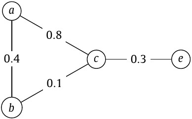
One of those problems is the spread of influence (or viral marketing) problem. We are given a social network with probabilistic influence relationships. Suppose Alexa has a probability of 0.8 to convince Claire to do something. We can model this with a node that symbolises Alexa and a node that symbolises Claire, and an edge pointing from Alexa to Claire, labelled with probability 0.8.
In this network, we assume all influence relationships to be symmetric. Hence, there is an edge with label 0.8 pointing from node a (Alexa) to node c (Claire), and the same arrow pointing back, resulting in one undirected edge connecting these two nodes.
Suppose now that we are a company planning a marketing campaign to promote our product. We want to use a word-of-mouth strategy on the probabilistic social network that we have of our potential customers. The way to start the process is to give free samples of our product to certain people in the network, and hope that they like it and convince their friends to buy the product, who then convince their friends, and so on, until our product goes viral. We have a limited budget for this (the constraint), and want to maximise the expected number of people who will eventually buy our product (the optimisation criterion). Which people in the network should get a free sample of our product?
Alternatively, we can require that the expected number of people who become customers exceeds a certain threshold (the constraint), while we aim to minimise the number of free samples that are distributed (the optimisation criterion). In practice, we can solve a stochastic constraint optimisation problem with a stochastic optimisation criterion and a budget constraint by formulating it as a stochastic constraint satisfaction problem (CSP) with a stochastic constraint and budget constraint. We then start the solving process with a very low threshold for the stochastic constraint (e.g., 0), and increase it each time we find a solution to the CSP. Then, we continue the search for a better solution until no better solution can be found. By then, the last solution we have found is an optimum solution.
Finding an optimum solution is hard
It is the stochastic constraint mentioned above that makes it hard to find a solution to SCPs. Given a strategy (a choice for which people receive a free sample), computing the probability that a person will become one of our customers is expensive. It involves summing probabilities over many, often partially overlapping, paths in the network. We then have to do this for all people in the network (to get the expected number of customers), and potentially have to repeat this for all possible strategies, in order to find a strategy that maximises the expected number of customers (by repeatedly finding an expected number of customers that exceeds an ever-increasing threshold of the stochastic constraint).
Joining forces
To find a solution to the problem, we therefore need two things: a way to quickly reason about probabilities, and a way to traverse the search space of strategies intelligently. We can combine the technique of knowledge compilation with the paradigm of constraint programming to create data structures (specifically, decision diagrams) that capture information about probability distributions, such that we can quickly compute probabilities, and to create constraint propagation algorithms on those data structures, which prune the search space.
A constraint propagation algorithm helps to prune the search space by removing values from the domains of variables. In particular, it ensures that variable domains contain no values that would falsify the constraint(s) in which the variables are present. Comparing different approaches that combine knowledge compilation and constraint programming, we find that having a dedicated constraint propagation algorithm for stochastic constraints tends to yield shorter solving times than approaches that decompose stochastic constraints into small, linear constraints (for which propagators already exist). We attribute this to the fact that in the decomposition process, we lose information about the relationship between different variables that participate in the stochastic constraint. Hence, the pruning power of the propagation methods is less, and the solver cannot prune certain parts of the search space that do not contain any solutions.
Paper
You can learn more about different ways of combining knowledge compilation and constraint programming in our paper “Exact stochastic constraint optimisation with applications in network analysis”, which was published in Artificial Intelligence, vol 304, March 2022. Authors: Anna L.D. Latour, Behrouz Babaki, Daniël Fokkinga, Marie Anastacio, Holger H. Hoos, Siegfried Nijssen. Link: doi.org/10.1016/j.artint.2021.103650
After obtaining his BSc. in Artificial Intelligence and MSc. in Computer Science, Mike Huisman joined LIACS in March 2021 as a teaching Ph.D. candidate. He is part of the Reinforcement Learning Group at LIACS and has also joined the ADA group in November 2021.
His research is in the field of deep meta-learning, where the goal is to learn an efficient deep learning algorithm that can learn new tasks quickly (from a limited amount of data). This can democratize the use of deep learning by lowering the threshold for using powerful deep learning technologies in terms of required compute resources and data. He conducts his research under the supervision of Prof. Dr. A. Plaat and Dr. J.N. van Rijn.
On 29 July, I defended my bachelor thesis entitled “Parallel Algorithm Portfolios in Sparkle” after half a year of work following the project start in February 2021. For this project I was part of the ADA group and was supervised by Koen van der Blom and Holger Hoos.
In a parallel portfolio, a set of independent, non-communicating solvers solve problem instances in parallel. Within the thesis, insight is given into the design and implementation of parallel portfolios into Sparkle. Additionally, experiments show the validity of the implementation and the practical capabilities of parallel portfolios as implemented in Sparkle.
My work built on the existing platform created by the Sparkle development team. The thesis is of value to the platform since the state of the art is represented by a set of algorithms, and parallel algorithm portfolios allow for an easily accessible method to conduct experiments with such portfolios.
Below an example is outlined showing how parallel algorithm portfolios can be used in Sparkle. Once the platform is initialized, the needed components (problem instances, solvers) are added to Sparkle. Using these the portfolio can be constructed. With the constructed portfolio and a selection of instances, an experiment can be conducted. Finally, we generate a report that describes the used components and an empirical evaluation of the results from the experiment.
First results in the thesis suggest that parallelising up to 64 instances of a nondeterministic solver with different random seeds results in performance gains compared to lower numbers of instances. When using 128 solver instances performance is similar to 64 solver instances, and there no longer seems to be a benefit to using more solver instances. With 256 or more solver instances the overhead appears to increase and performance starts to drop again in this practical implementation.
If you are interested in the project, feel free to take a look at the bitbucket project page and try Sparkle for yourself.